This post is a practical answers from Problem set three part B on GSLIB book which aims to figure out how Data Configuration affect kriging estimation. Here, I just simply implement pygeostat and kb2b.exe to answer the questions. All of the comments comes from the book.
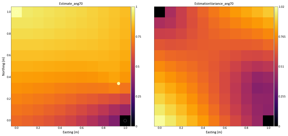
Introduction to Data Configuration Problem
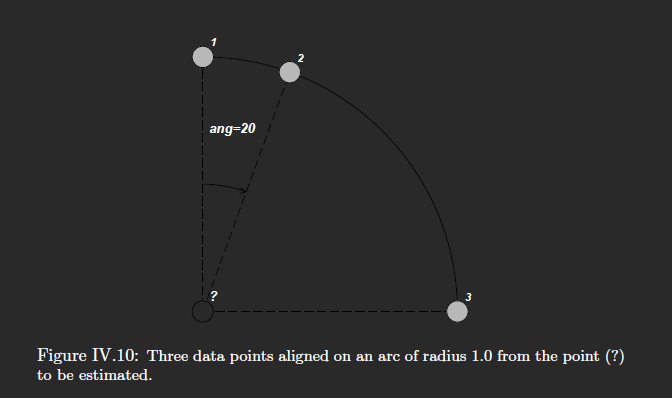
This part aims at developing intuition about the influence of the data configuration. Consider the situation shown in Figure IV.10 with the angle ang varying between 0o and 90o. Start with these data, an isotropic spherical variogram with a range of 2.0, a variance contribution of C = 0:8, and nugget constant C0 = 0:2, and use kb2d.exe to answer the questions.
# importing modules
import math
import numpy as np
import pandas as pd
import pygeostat as gs
# Importing data file
partb = gs.DataFile('partb.dat', x='Xloc', y='Yloc')_= gs.location_plot(partb, s=100)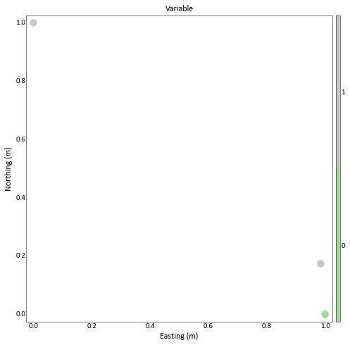
Question 1
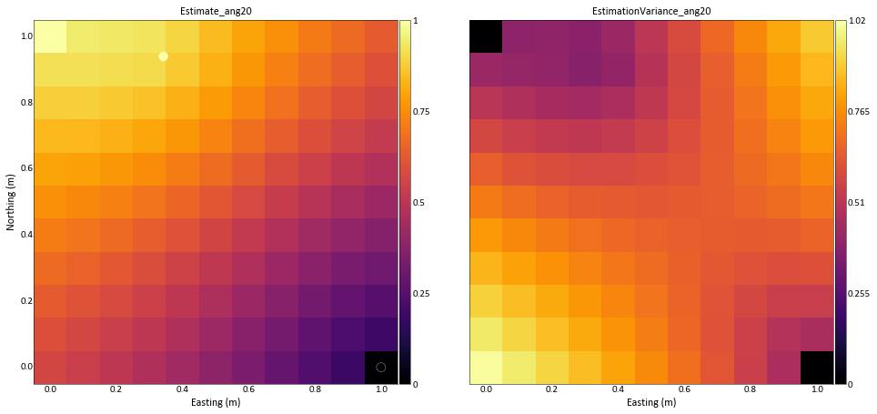
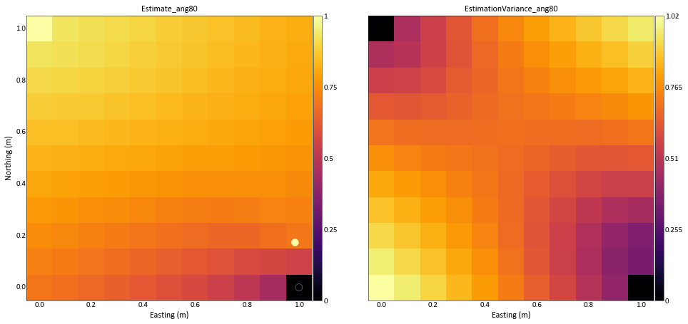
How does the weight applied to data point 2 vary with ang? Vary ang in 5 or 10 degree increments (you may want to customize the kriging program to recompute automatically the coordinates of the second data point). Plot appropriate graphs and comment on the results.
kb2d_p = gs.Program('kb2d')# Running Kriging Program on loop for different (x,y) location
for ang in np.arange(10,90,10):
x = math.sin(math.radians(ang)) # Calculating x location
y = math.cos(math.radians(ang)) # Calculating y location
partb.data.loc[0, 'Xloc'] = x # Replacing data with new x location
partb.data.loc[0, 'Yloc'] = y # Replacing data with new y location
gs.write_gslib(data=partb, flname='partb.dat', title='Part B: Example Data File') # Overwriting file with new (x,y) data
# Defining grid definition
my_griddef = gs.grid_definition.GridDef(grid_arr=[11, 0, 0.1,
11, 0, 0.1,
1, 0, 0.1])
# Defining parameters for KB2D program
parstr = f""" Parameters for KB2D
*******************
START OF PARAMETERS:
{partb.flname} -file with data
1 2 3 -columns for X, Y, and variable
-5 5 -trimming limits
1 -debugging level: 0,1,2,3
kb2d.dbg -file for debugging output
kb2d.out -file for kriged output
11 0 0.1 -nx,xmn,xsiz
11 0 0.1 -ny,ymn,ysiz
1 1 -x and y block discretization
1 4 -min and max data for kriging
12.0 -maximum search radius
1 2.302 -0=SK, 1=OK, (mean if SK)
1 0.2 -nst, nugget effect
1 0.8 0.0 2.0 2.0 -it, c, azm, a_max, a_min
"""
# Running the program
kb2d_p.run(parstr=parstr, quiet=True, liveoutput=False)
partb_kb2d = gs.DataFile('kb2d.out', griddef=my_griddef)
# Plotting estimation
fig, ax = gs.subplots(1,2, figsize=(16,16), cbar_mode='each')
_ = gs.slice_plot(data=partb_kb2d, ax=ax[0], var='Estimate', title=f'Estimate_ang{ang}', griddef=my_griddef, pointdata=partb, pointvar='Variable', cmap='inferno', pointkws={'edgecolors':'white', 's':100})
_ = gs.slice_plot(data=partb_kb2d, ax=ax[1], var='Estimation Variance', title=f'EstimationVariance_ang{ang}', griddef=my_griddef, cmap='inferno')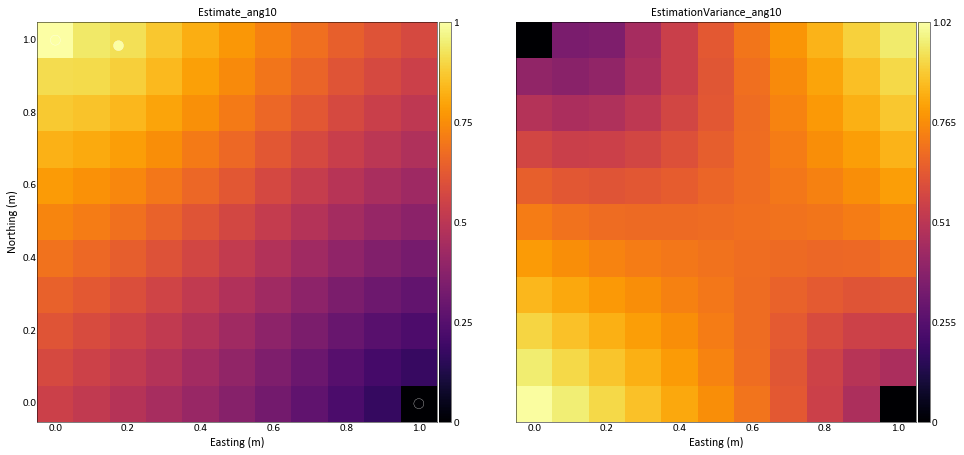
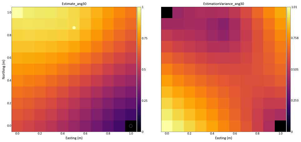
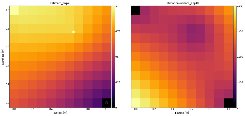
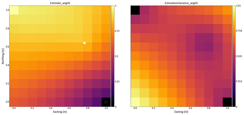
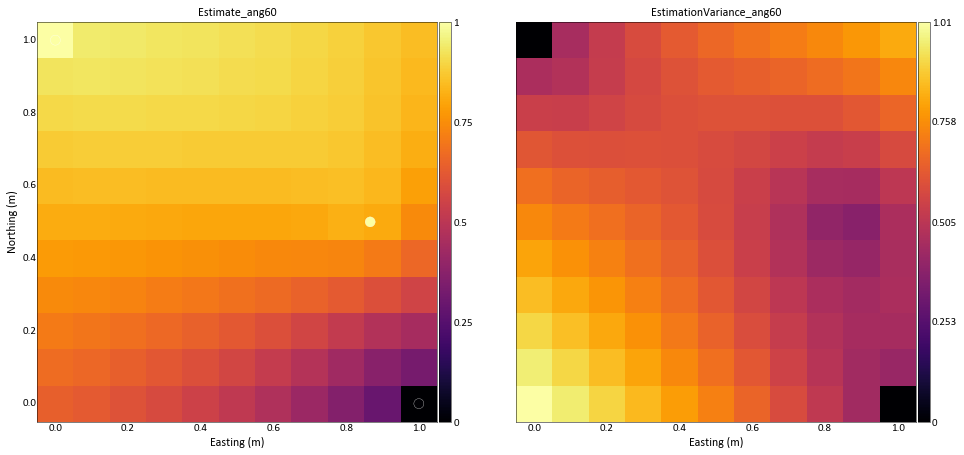
np.arange(0,90,10)array([ 0, 10, 20, 30, 40, 50, 60, 70, 80])
Comment:
- The proposed configuration is symmetric about the 45o line. As the second point approaches either endpoint, the redundancy with the far point decreases and the redundancy with the near point increases. The rate of increase and decrease of the kriging weight differs depending on the variogram model. In the first case (low nugget effect C0 = 0:1) the increase in redundancy with the near point is less than the decrease in redundancy with the far point; hence, the weight attributed to the second point increases as the point nears an endpoint.
Question 2
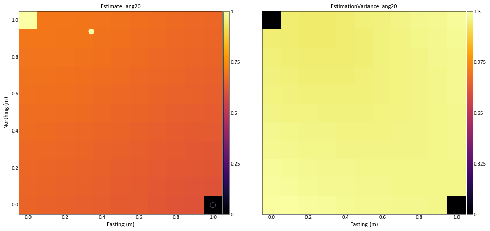
Repeat question 1 with C0 = 0:9 and C = 0:1.
# Running Kriging Program on loop for different (x,y) location
for ang in np.arange(10,90,10):
    x = math.sin(math.radians(ang))             # Calculating x location
    y = math.cos(math.radians(ang))             # Calculating y location

    partb.data.loc[0, 'Xloc'] = x               # Replacing data with new x location
    partb.data.loc[0, 'Yloc'] = y               # Replacing data with new y location

    gs.write_gslib(data=partb, flname='partb.dat', title='Part B: Example Data File')     # Overwriting file with new (x,y) data

    # Defining grid definition
    my_griddef = gs.grid_definition.GridDef(grid_arr=[11, 0, 0.1,
                                                      11, 0, 0.1,
                                                      1, 0, 0.1])

    # Defining parameters for KB2D program
    parstr = f"""     Parameters for KB2D
                      *******************

    START OF PARAMETERS:
    {partb.flname}               -file with data
    1    2   3                   -columns for X, Y, and variable
    -5   5                       -trimming limits
    1                            -debugging level: 0,1,2,3
    kb2d.dbg                     -file for debugging output
    kb2d.out                     -file for kriged output
    11   0     0.1               -nx,xmn,xsiz
    11   0     0.1               -ny,ymn,ysiz
    1    1                       -x and y block discretization
    1    4                       -min and max data for kriging
    12.0                         -maximum search radius
    1    2.302                   -0=SK, 1=OK,  (mean if SK)
    1    0.9                     -nst, nugget effect
    1    0.1  0.0  2.0  2.0      -it, c, azm, a_max, a_min
    """
    # Running the program
    kb2d_p.run(parstr=parstr, quiet=True, liveoutput=False)
    partb_kb2d = gs.DataFile('kb2d.out', griddef=my_griddef)

    # Plotting estimation
    fig, ax = gs.subplots(1,2, figsize=(16,16), cbar_mode='each')
    _ = gs.slice_plot(data=partb_kb2d, ax=ax[0], var='Estimate', title=f'Estimate_ang{ang}', griddef=my_griddef, pointdata=partb, pointvar='Variable', pointkws={'edgecolors':'white', 's':100}, cmap='inferno')
    _ = gs.slice_plot(data=partb_kb2d, ax=ax[1], var='Estimation Variance', title=f'EstimationVariance_ang{ang}', griddef=my_griddef,  cmap='inferno')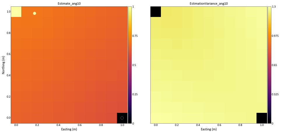
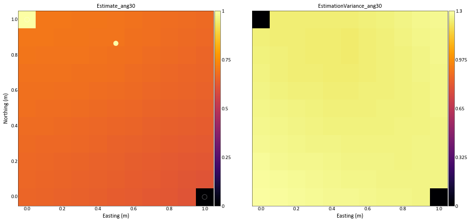
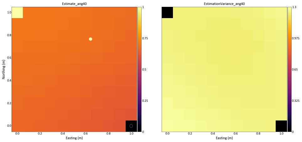
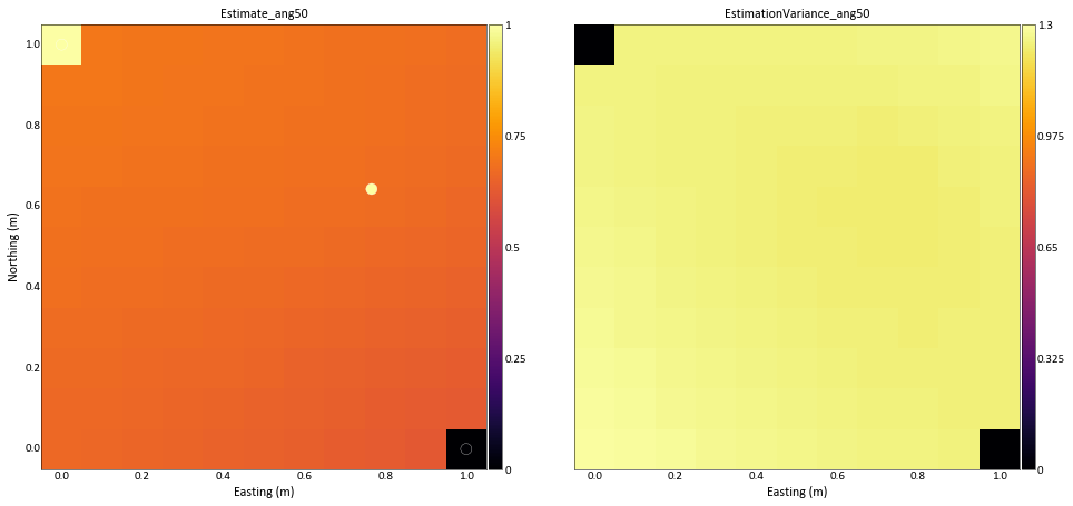
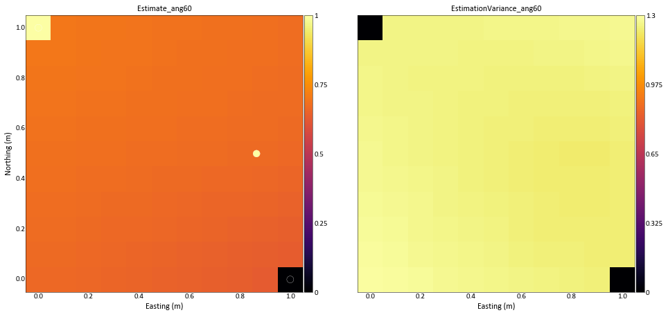
Comment:
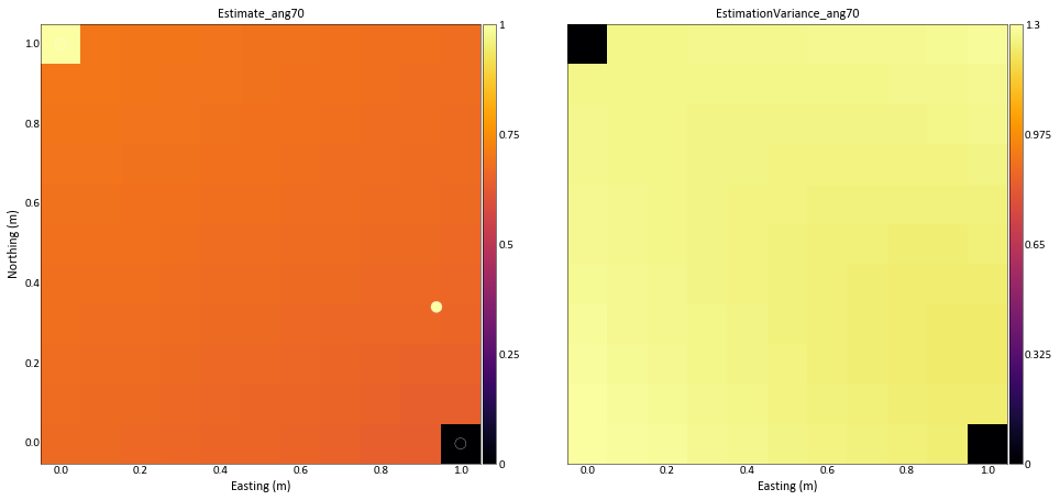
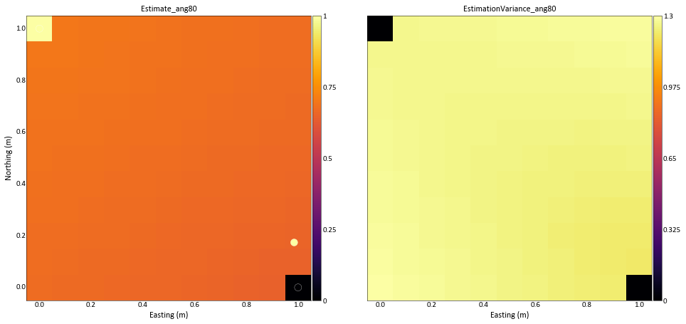
- With a high nugget effect (C0 = 0:9) the increase in redundancy with the near point is greater than the decrease in redundancy with the far point; hence, the weight decreases as the point nears an endpoint. All the kriging weights in this case are almost equal.
Reference
- Deutsch, C. V., & Journel, A. G. (1998). GSLIB: Geostatistical software library and user’s guide. New York: Oxford University Press.
- Pygeostat Documentation. http://www.ccgalberta.com/pygeostat/welcome.html