One thing that’s always bothered me when learning resource estimation: finding public drill hole data is surprisingly hard. Company data is confidential — which is fair. But if you just want to practice, using real data carries too much risk.
So I made my own. Synthetic, reproducible, and free for anyone to use.
This dataset has also been used in some experiments I wrote about previously.
I wanted something that made geological sense. Nickel laterite has a distinct vertical profile — from overburden at surface, down through limonite into saprolite, then bedrock. Each zone has different grade characteristics.
Surface
  ↓
┌─────────────────────┐
│  Overburden (0-3m)  │  Soil, root zone
├─────────────────────┤
│  LIMONITE (3-12m)   │  Rich in Fe, Co, Mn
│  Ni: 0.5-1.5%       │  Fe: 30-50%
│                     │  Low MgO (leached)
├─────────────────────┤
│  SAPROLITE (4-18m)  │  Rich in Ni, MgO
│  Ni: 1.5-4%         │  Fe: 10-25%
│                     │  Mining target
├─────────────────────┤
│  BEDROCK            │  Fresh peridotite
└─────────────────────┘
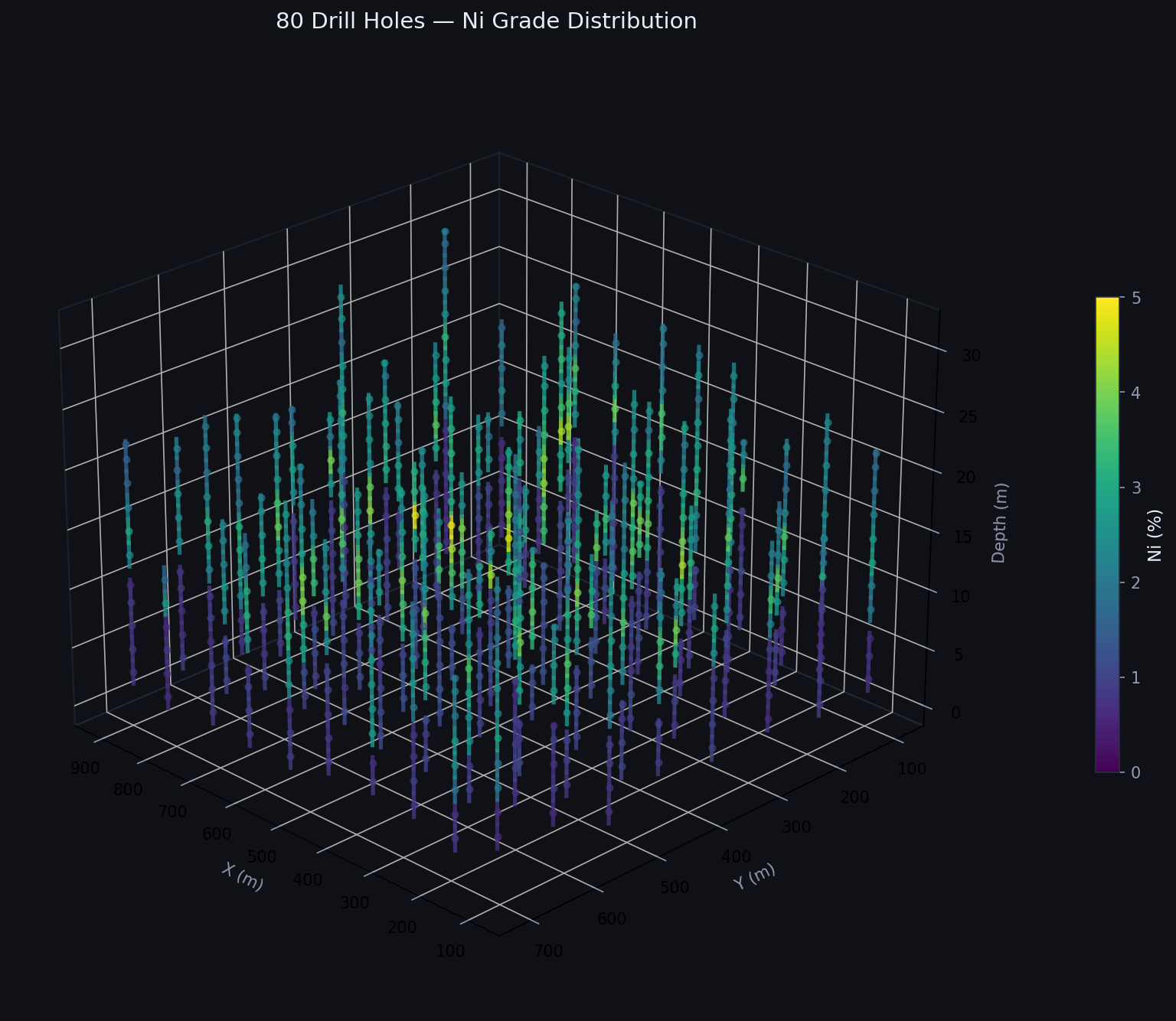
Five things I modeled: Ni increasing with depth (supergene enrichment), high Fe in limonite (iron cap), low MgO in limonite due to leaching, Co associating with Mn-oxides, and spatial autocorrelation — nearby holes having similar grades.
The code is straightforward. Seed 42 for reproducibility, 80 drill holes on a 10×8 grid, roughly 800×600 meters. ±5m jitter simulates real survey imprecision.
import csv, math, random
random.seed(42)

N_HOLES = 80
SAMPLE_INTERVAL = 2.0
DEPOSIT_CENTER = (500, 400)
The most interesting part was the spatial trend. Nickel laterite deposits are lenticular — grades peak at the center and taper off toward the edges. A Gaussian function does the job:
def spatial_factor(x, y, weight=0.3):
    dx = (x - 500) / 300
    dy = (y - 400) / 250
    dist_sq = dx*dx + dy*dy
    gauss = math.exp(-0.5 * dist_sq)
    return 1.0 + weight * (gauss - 0.5) * 2
The first time I ran this and saw that center holes actually got higher grades — surprisingly satisfying. weight=0.3 means spatial influence accounts for roughly 30% of grade variation. The rest comes from other factors.
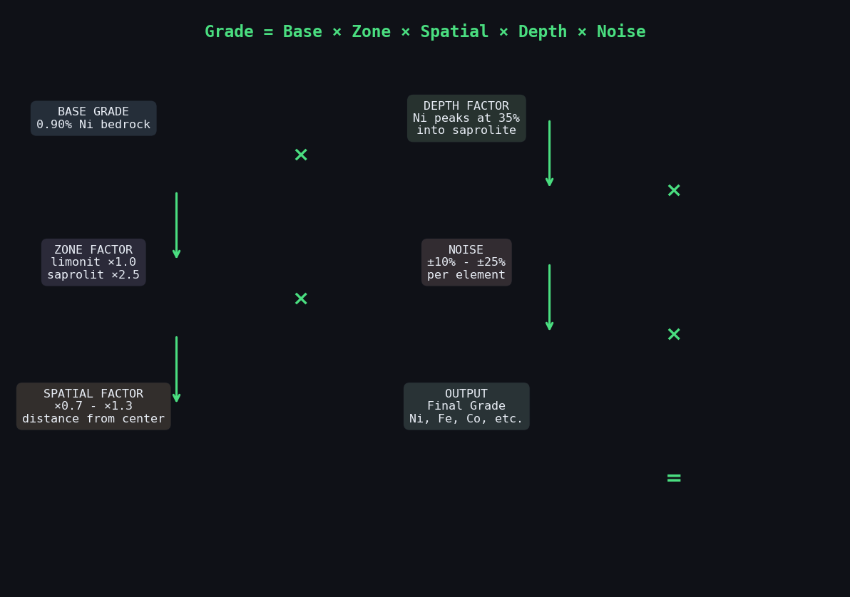
The core function — generate_grade() — combines base grade, zone factor (limonite vs saprolite), spatial factor, depth factor, and noise. Each element gets its own parameters based on its geochemical behavior.
The logic: multiply base by zone factor, then spatial factor, then depth factor, then add noise. Ni in limonite gets ×1.0 (stable), in saprolite ×2.5 (supergene enrichment). Fe works the opposite way — high in limonite (iron cap), low in saprolite.
| Element | Base | Limonite | Saprolite | Noise |
|---|---|---|---|---|
| Ni | 0.90% | 1.0× | 2.5× | 20% |
| Fe | 25% | 1.4× | 0.6× | 15% |
| Co | 0.04% | 1.8× | 0.5× | 25% |
| MgO | 20% | 0.4× | 1.5× | 15% |
The result: 808 assay samples from 80 drill holes. Limonite Ni averages 0.93%, saprolite Ni averages 2.67%. Reasonable for typical laterite deposits.
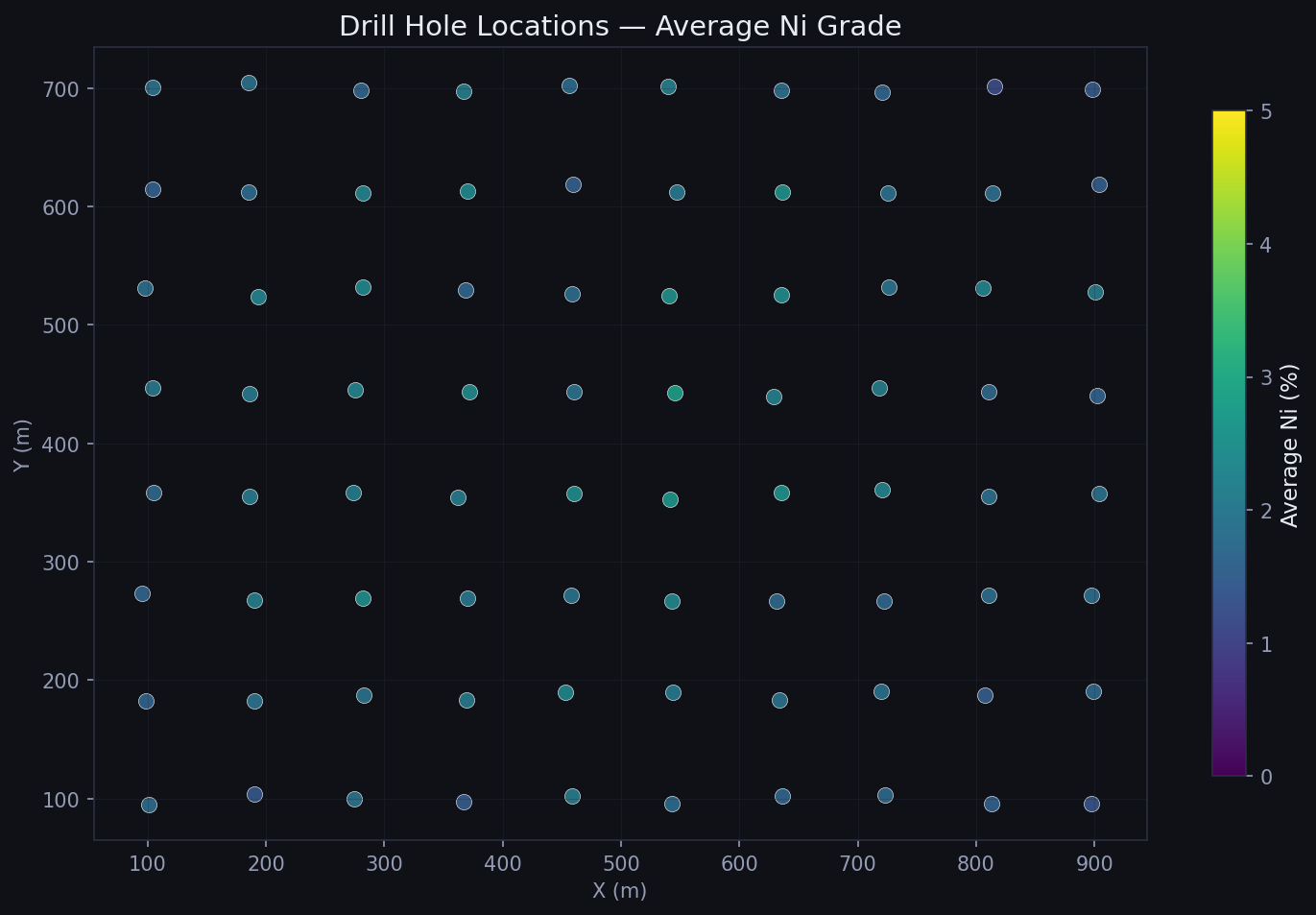
The plan view shows the spatial pattern clearly — center holes (DH-036, DH-046, DH-047 area) have higher grades. That’s the spatial trend at work.
Highest Ni samples, all in saprolite:
- DH-046 | 14.6m | Ni=4.86%
- DH-047 | 14.0m | Ni=4.76%
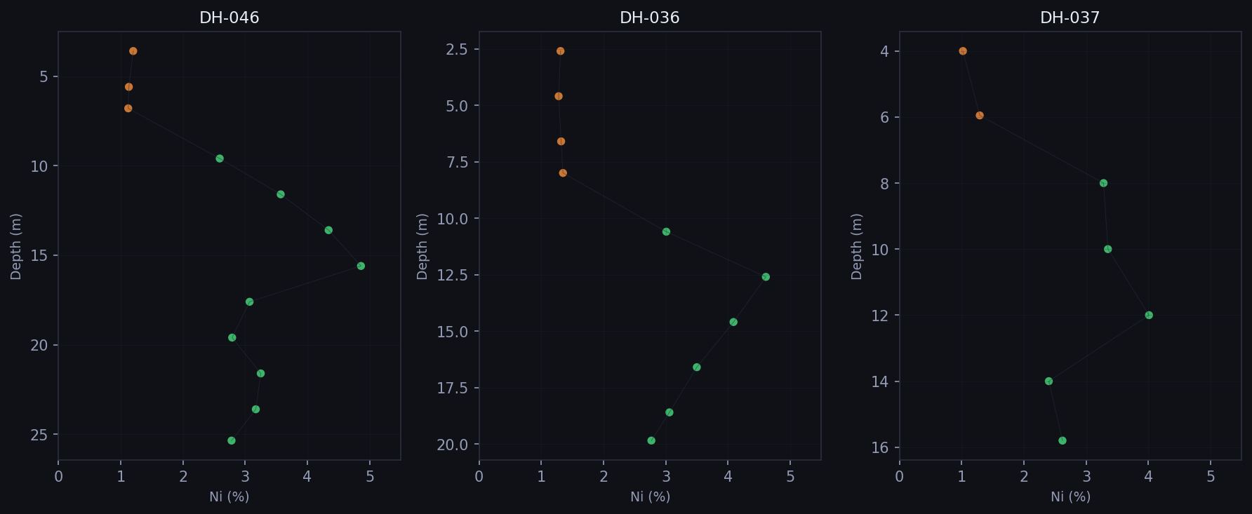
One thing I found interesting: Ni in saprolite doesn’t increase linearly with depth. It peaks at around 35% into the zone, then drops toward bedrock. This matches real supergene enrichment behavior, so I made sure the model captured it.
To try it yourself:
Notebook: pip install jupyter ipywidgets matplotlib then run notebooks/generate_nickel_data.py. Preset or manual mode.
CLI: python3 scripts/generator_engine.py sulawesi_hp output/
Download CSV: Sample output (Sulawesi HP)
The generator produces 4 tables: collar, assay, survey, and topography. Topography uses Fourier synthesis — actual hills and valleys, not a flat surface.
Three presets:
- Sulawesi HP: Steep relief, 100m grid
- Halmahera LP: Thick limonite, gentle relief
- Gag Island: Flat, tight grid, ultra-high Ni