This post is a practical answers from Problem set three part A on GSLIB book which aims to figure out how variogram parameters affect kriging estimation. Here, I just simply implement pygeostat and kb2b.exe to answer the questions. All of the comments comes from the book.
Introduction to The Problem
When performing a kriging study, it is good practice to select one or two representative locations and have a close look at the kriging solution including the kriging matrix, the kriging weights, and how the estimate compares to nearby data. This part of the problem set consists of estimating point unsampled location using Ordinary Kriging with different variogram parameters. The goal is to gain an intuitive understanding of the relative importance of the various variogram parameters. Note in most cases a standardized semivariogram is used such that the nugget constant C0 plus the variance contributions of all nested structures sum to 1.0.
# importing modules
import numpy as np
import pandas as pd
import pygeostat as gs
# importing data and displaying data tables
parta = gs.DataFile('parta.dat', x= 'Xloc', y= 'Yloc', variables=['Variable', 'Normal Scores'])
print(parta.data)Xloc Yloc Variable Normal Scores 0 38.5 28.5 0.574 -0.493 1 45.5 29.5 1.211 0.517 2 41.5 26.5 2.127 0.461 3 39.5 31.5 8.340 1.483 4 38.5 31.5 18.642 2.119 5 39.5 30.5 7.938 1.439 6 39.5 32.5 2.284 0.515 7 40.5 31.5 2.509 0.603
# plotting data
_ = gs.location_plot(parta, var='Normal Scores', s=100)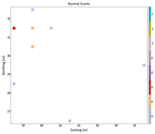
# statistical summary of the data
print(parta.describe())
Variable Normal Scores count 8.000000 8.000000 mean 5.453125 0.830500 std 6.094856 0.810117 min 0.574000 -0.493000 25% 1.898000 0.501500 50% 2.396500 0.560000 75% 8.038500 1.450000 max 18.642000 2.119000
# inferring grid definition from the data
parta_griddef = parta.infergriddef(blksize=[1,1, None])
parta_griddef
Pygeostat GridDef: 18 33.5 1.0 17 21.5 1.0 1 0.5 1.0
Question 1
Consider an isotropic spherical variogram with a range of 10 plus a nugget effect. Vary the relative nugget constant from 0.0 (i.e., C0 = 0:0 and C = 1:0) to 1.0 (i.e., C0 = 1:0 and C = 0:0) in increments of 0.2.
kb2d_p = gs.Program('kb2d')for nugget in[0, 0.2, 0.4, 0.6, 0.8, 1]:
parstr = f""" Parameters for KB2D
*******************
START OF PARAMETERS:
{parta.flname} -file with data
1 2 4 -columns for X, Y, and variable
-1.0e21 1.0e21 -trimming limits
2 -debugging level: 0,1,2,3
kb2d_nugget_{nugget}.dbg -file for debugging output
kb2d_nugget_{nugget}.out -file for kriged output
18 33.5 1.0 -nx,xmn,xsiz
17 21.5 1.0 -ny,ymn,ysiz
1 1 -x and y block discretization
7 20 -min and max data for kriging
40.0 -maximum search radius
1 5.453 -0=SK, 1=OK, (mean if SK)
1 {nugget} -nst, nugget effect
1 {1 - nugget} 0.0 10.0 10.0 -it, c, azm, a_max, a_min
"""
kb2d_p.run(parstr=parstr, liveoutput=False, quiet=True)
parta_kb2d = gs.DataFile(f'kb2d_nugget_{nugget}.out', griddef=parta_griddef)
fig, ax = gs.subplots(1,2, figsize=(16,16), cbar_mode='each')
gs.slice_plot(data=parta_kb2d, ax=ax[0], var='Estimate', title=f'Estimate_nugget_{nugget}', griddef=parta_griddef, pointdata=parta, pointvar='Normal Scores', pointkws={'edgecolors':'k', 's':100})
gs.slice_plot(data=parta_kb2d, ax=ax[1], var='Estimation Variance', title=f'EstimationVariance_nugget_{nugget}', griddef=parta_griddef)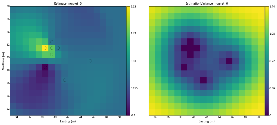
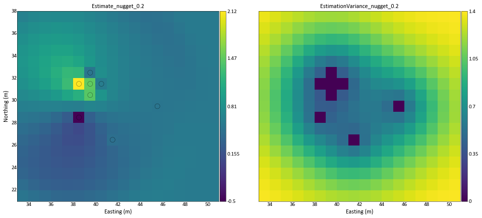
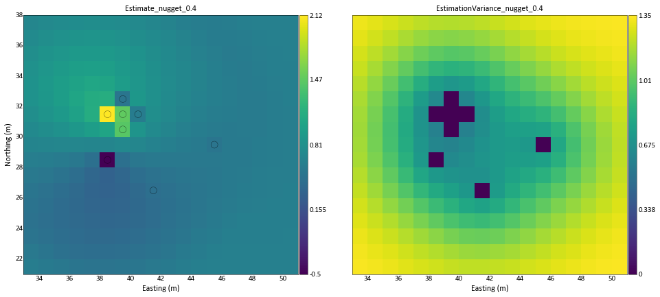
Comment on Relative nugget effect:
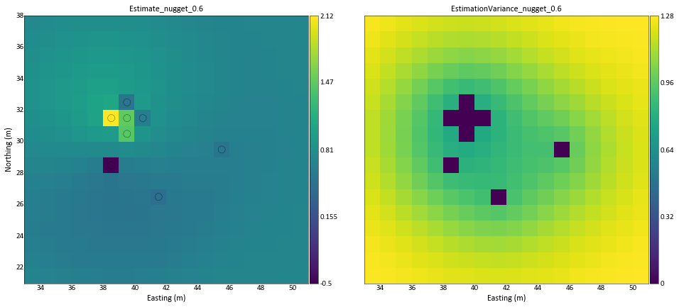
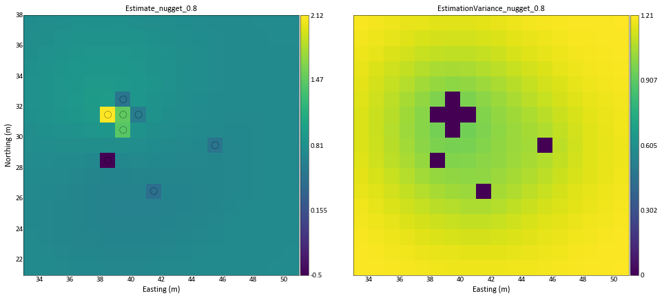
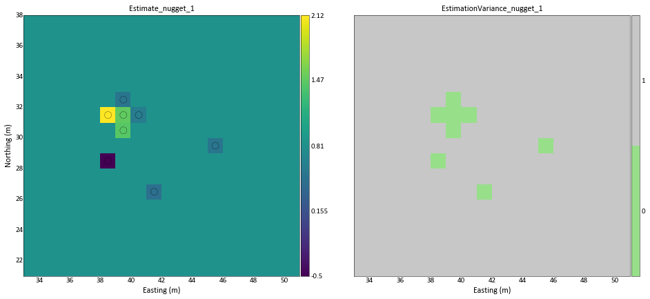
When the relative nugget effect is small, the data redundancy and the proximity to the point being estimated become important. This implies that close samples are weighted more and samples within clusters are treated as less informative. A low relative nugget effect may cause a wider variation in the weights (from negative to greater than one in some cases), which may cause outlier data values to be more problematic. No general comment can be made about the magnitude of the estimate, although a surface estimated with a large nugget effect will be smoother.
Question 2
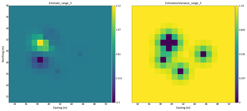
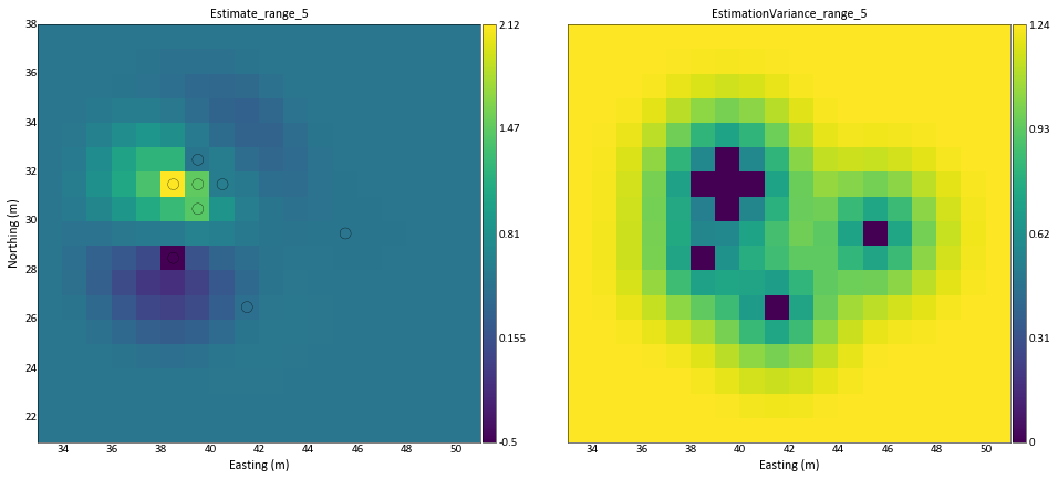
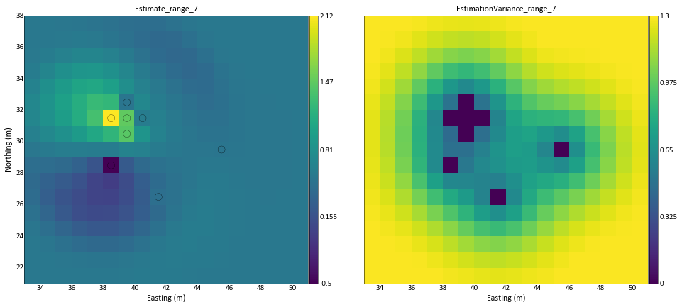
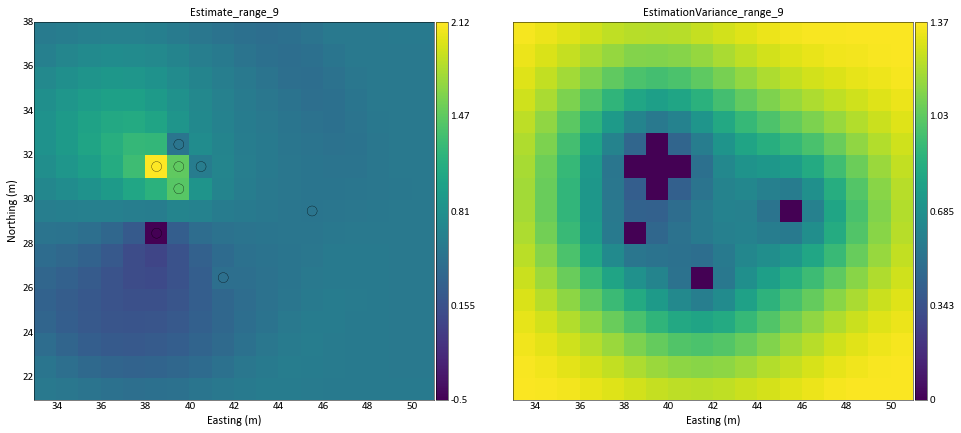
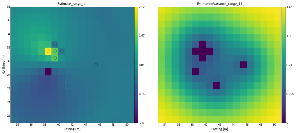
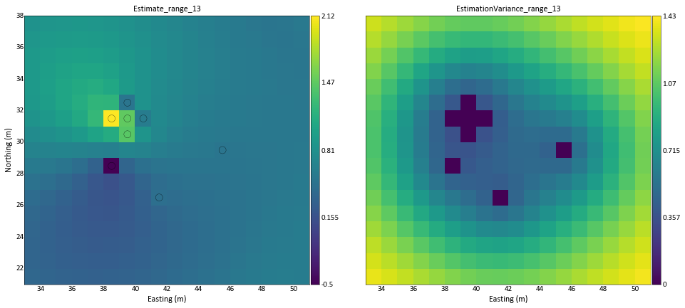
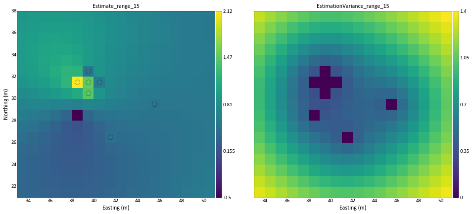
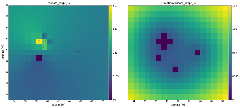
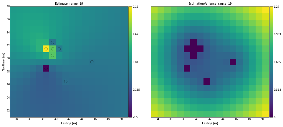
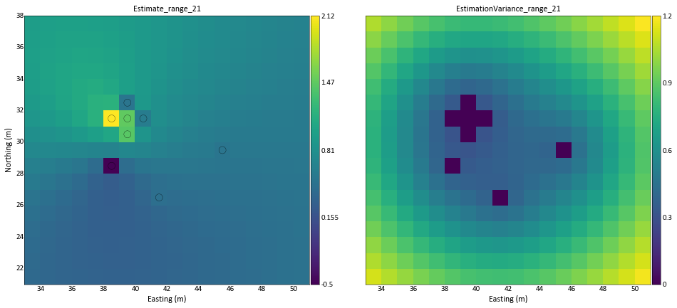
Consider an isotropic spherical variogram with a variance contribution C = 0:8 and nugget constant C0 = 0:2. Vary the isotropic range from 1.0 to 21.0 in increments of 2.0.
for range_ in np.arange(1,22, 2):
    parstr = f"""      Parameters for KB2D
                      *******************

    START OF PARAMETERS:
    {parta.flname}                         -file with data
    1   2   4                              -   columns for X, Y, and variable
    -1.0e21   1.0e21                       -   trimming limits
    2                                      -debugging level: 0,1,2,3
    kb2d_range_{range_}.dbg                -file for debugging output
    kb2d_range_{range_}.out                -file for kriged output
    18    33.5  1.0                        -nx,xmn,xsiz
    17    21.5  1.0                        -ny,ymn,ysiz
    1    1                                 -x and y block discretization
    7    20                                -min and max data for kriging
    40.0                                   -maximum search radius
    1    5.453                             -0=SK, 1=OK,  (mean if SK)
    1   0.2                                -nst, nugget effect
    1   0.8  0.0  {range_}  {range_}       -it, c, azm, a_max, a_min
    """
    kb2d_p.run(parstr=parstr, liveoutput=False, quiet=True)

    parta_kb2d = gs.DataFile(f'kb2d_range_{range_}.out', griddef=parta_griddef)
    fig, ax = gs.subplots(1,2, figsize=(16,16), cbar_mode='each')
    gs.slice_plot(data=parta_kb2d, ax=ax[0], var='Estimate', title=f'Estimate_range_{range_}', griddef=parta_griddef, pointdata=parta,pointvar='Normal Scores', pointkws={'edgecolors':'k', 's':100})
    gs.slice_plot(data=parta_kb2d, ax=ax[1], var='Estimation Variance', title=f'EstimationVariance_range_{range_}', griddef=parta_griddef)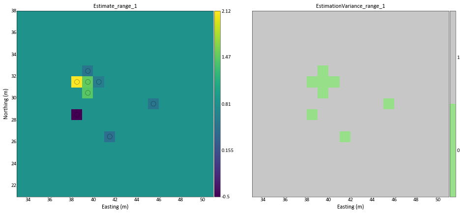
Comment on Range:
When the range is smaller than the interdistance between any two data points, then the situation is equivalent to a pure nugget effect model. As the range increases, the continuity increases, causing the proximity to the estimated location and data redundancy to become important. As the range becomes very large with a nugget effect, then the estimation is equivalent to a pure nugget system; if there is no nugget effect, then the kriging system behaves as if a linear variogram model were chosen.
Question 3
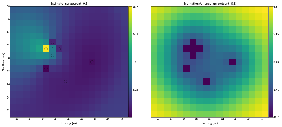
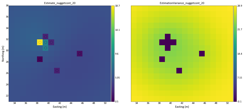
Consider an isotropic spherical variogram with a range of 12.0. Vary the nugget constant and variance contribution values without changing their relative proportions [i.e., keep C0=(C0 + C) = 0:2]. Try C0 = 0:2 (C = 0:8), C0 = 0:8 (C = 3:2), and C0 = 20:0 (C = 80:0).
for nuggetcont in [0.2, 0.8, 20]:
    variancecont = ((nugget/0.2) - nugget)
    parstr = f"""      Parameters for KB2D
                      *******************

    START OF PARAMETERS:
    {parta.flname}                         -file with data
    1   2   3                              -   columns for X, Y, and variable
    -1.0e21   1.0e21                       -   trimming limits
    2                                      -debugging level: 0,1,2,3
    kb2d_nuggetcont_{nuggetcont}.dbg                -file for debugging output
    kb2d_nuggetcont_{nuggetcont}.out                -file for kriged output
    18    33.5  1.0                        -nx,xmn,xsiz
    17    21.5  1.0                        -ny,ymn,ysiz
    1    1                                 -x and y block discretization
    7    20                                -min and max data for kriging
    40.0                                   -maximum search radius
    1    5.453                             -0=SK, 1=OK,  (mean if SK)
    1   {nuggetcont}                                -nst, nugget effect
    1   {variancecont}  0.0  12  12                   -it, c, azm, a_max, a_min
    """
    kb2d_p.run(parstr=parstr, liveoutput=False, quiet=True)

    parta_kb2d = gs.DataFile(f'kb2d_nuggetcont_{nuggetcont}.out', griddef=parta_griddef)
    fig, ax = gs.subplots(1,2, figsize=(16,16), cbar_mode='each')
    gs.slice_plot(data=parta_kb2d, ax=ax[0], var='Estimate', title=f'Estimate_nuggetcont_{nuggetcont}', griddef=parta_griddef, pointdata=parta,pointvar='Variable', pointkws={'edgecolors':'k', 's':100})
    gs.slice_plot(data=parta_kb2d, ax=ax[1], var='Estimation Variance', title=f'EstimationVariance_nuggetcont_{nuggetcont}', griddef=parta_griddef)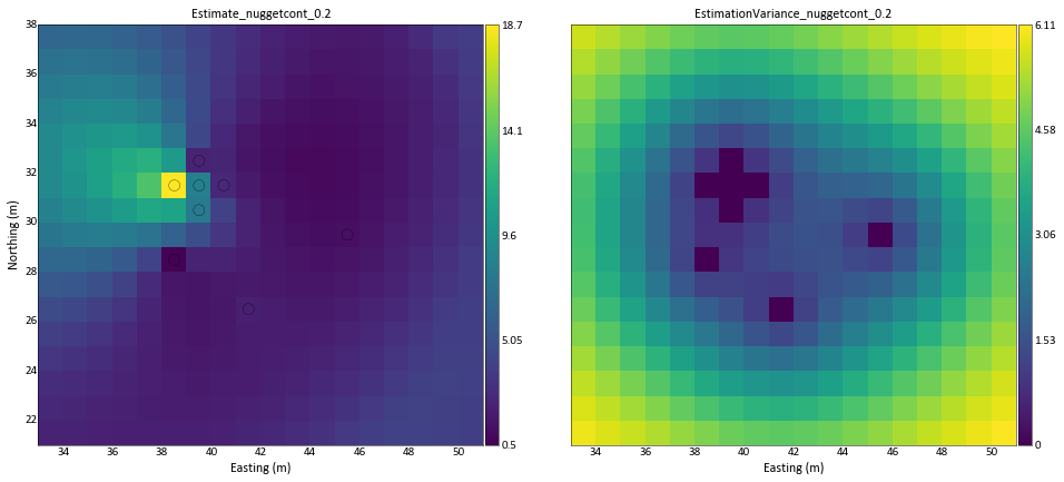
Comment on Scale:
The scaling of the variogram affects only the kriging (estimation) variance; only the relative shape of the variogram determines the kriging weights and estimate.
Question 4
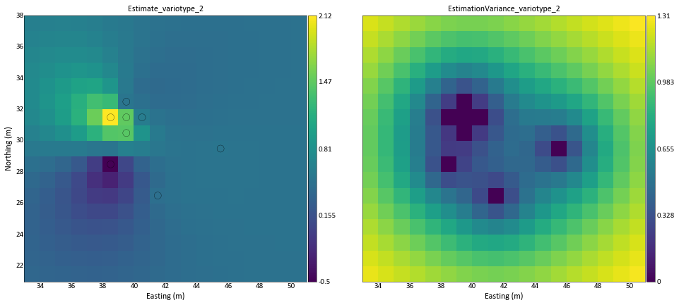
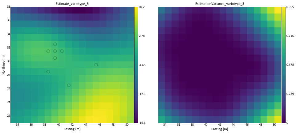
Consider alternative isotropic variogram models with a variance contribution C = 1:0 and nugget constant C0 = 0:0. Keep the range constant at 15. Consider the spherical, exponential, and Gaussian variogram models. Prepare a table showing the kriging weight applied to each datum, the kriging estimate, and the kriging variance. Use the programs vmodel and vargplt to plot the variogram models if you are unfamiliar with their shapes.
for variotype in [1, 2, 3]:
    parstr = f"""      Parameters for KB2D
                      *******************

    START OF PARAMETERS:
    {parta.flname}                         -file with data
    1   2   4                              -   columns for X, Y, and variable
    -1.0e21   1.0e21                       -   trimming limits
    2                                      -debugging level: 0,1,2,3
    kb2d_variotype_{variotype}.dbg                -file for debugging output
    kb2d_variotype_{variotype}.out                -file for kriged output
    18    33.5  1.0                        -nx,xmn,xsiz
    17    21.5  1.0                        -ny,ymn,ysiz
    1    1                                 -x and y block discretization
    7    20                                -min and max data for kriging
    40.0                                   -maximum search radius
    1    5.453                             -0=SK, 1=OK,  (mean if SK)
    1   0.0                                -nst, nugget effect
    {variotype}   1  0.0  15  15                   -it, c, azm, a_max, a_min
    """
    kb2d_p.run(parstr=parstr, liveoutput=False, quiet=True)

    parta_kb2d = gs.DataFile(f'kb2d_variotype_{variotype}.out', griddef=parta_griddef)
    fig, ax = gs.subplots(1,2, figsize=(16,16), cbar_mode='each')
    gs.slice_plot(data=parta_kb2d, ax=ax[0], var='Estimate', title=f'Estimate_variotype_{variotype}', griddef=parta_griddef, pointdata=parta,pointvar='Normal Scores', pointkws={'edgecolors':'k', 's':100})
    gs.slice_plot(data=parta_kb2d, ax=ax[1], var='Estimation Variance', title=f'EstimationVariance_variotype_{variotype}', griddef=parta_griddef)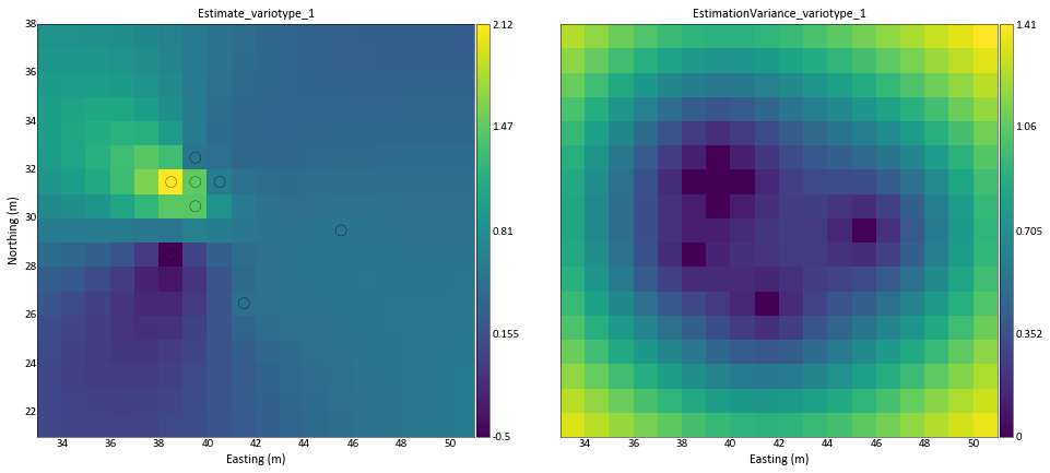
Comment on Shape:
Both the exponential and spherical variograms have a linear shape near the origin. The exponential model growth from the origin is steeper, causing it to behave in a manner similar to a shorter-range spherical model. The Gaussian model is parabolic near the origin, indicating a spatially very continuous variable. This may cause very large positive and negative weights (which are entirely reasonable given such continuity). If the actual data values are not extremely continuous and a Gaussian model is used, then erratic results can arise from the negative weights. Numerical precision problems also arise because of off-diagonal elements that have nearly zero variogram (maximum covariance) values. The problem is not so much the shape of the variogram as the lack of a nugget. The addition of a nugget does not change appreciably the shape of the variogram but improves numerical stability.
Question 5
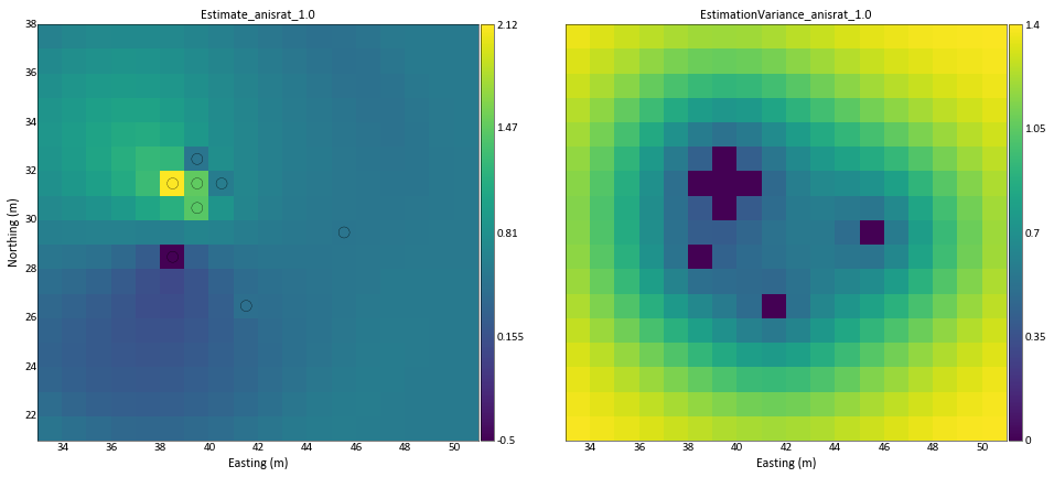
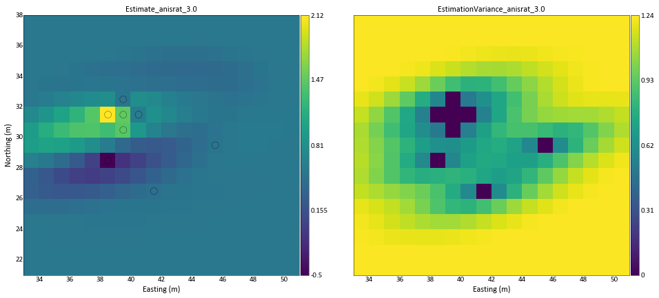
Consider a spherical variogram with a long range of 10.0, a variance contribution C = 0:8, and nugget constant C0 = 0:2. Consider a geometric anisotropy with the direction of major continuity at 75 degrees clockwise from the y axis and anisotropy ratios of 0.33, 1.0, and 3.0. Prepare a table showing the kriging weight applied to each datum, the kriging estimate, and the kriging variance. Comment on the results.
for anisrat in [0.33, 1.0, 3.0]:
    a_min = 10/anisrat
    parstr = f"""      Parameters for KB2D
                      *******************

    START OF PARAMETERS:
    {parta.flname}                         -file with data
    1   2   4                              -   columns for X, Y, and variable
    -1.0e21   1.0e21                       -   trimming limits
    2                                      -debugging level: 0,1,2,3
    kb2d_anisrat_{anisrat}.dbg                -file for debugging output
    kb2d_anisrat_{anisrat}.out                -file for kriged output
    18    33.5  1.0                        -nx,xmn,xsiz
    17    21.5  1.0                        -ny,ymn,ysiz
    1    1                                 -x and y block discretization
    7    20                                -min and max data for kriging
    40.0                                   -maximum search radius
    1    5.453                             -0=SK, 1=OK,  (mean if SK)
    1   0.2                                -nst, nugget effect
    1   0.8  75  10  {a_min}                   -it, c, azm, a_max, a_min
    """
    kb2d_p.run(parstr=parstr, liveoutput=False, quiet=True)

    parta_kb2d = gs.DataFile(f'kb2d_anisrat_{anisrat}.out', griddef=parta_griddef)
    fig, ax = gs.subplots(1,2, figsize=(16,16), cbar_mode='each')
    gs.slice_plot(data=parta_kb2d, ax=ax[0], var='Estimate', title=f'Estimate_anisrat_{anisrat}', griddef=parta_griddef, pointdata=parta,pointvar='Normal Scores', pointkws={'edgecolors':'k', 's':100})
    gs.slice_plot(data=parta_kb2d, ax=ax[1], var='Estimation Variance', title=f'EstimationVariance_anisrat_{anisrat}', griddef=parta_griddef)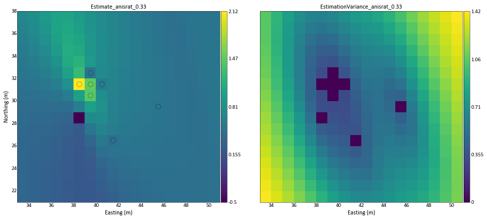
Comment on Anisotropy:
The anisotropy factor may be applied to the range of the variogram, or equivalently to the coordinates (after rotation to identify the main directions of continuity). It is instructive to think of geometric anisotropy as a geometric correction to the coordinates followed by application of an isotropic model.
Reference
- Deutsch, C. V., & Journel, A. G. (1998). GSLIB: Geostatistical software library and user’s guide. New York: Oxford University Press.
- Pygeostat Documentation. http://www.ccgalberta.com/pygeostat/welcome.html